Fixed
and variable costs
Possibly of even greater importance than the distinction between capital
costs and operating costs is the distinction between fixed
costs and variable costs. You will see that the main argument
for the cost-efficiency of ODL - the expectation that distance learning
generates economies of scale - rests on this distinction.
The
distinction relates to volume of activity. The principal activities of
an ODL institution consists in teaching students. Hence fixed costs
are those which do not increase with the volume of activity, i.e. the
number of students taught. Development costs of teaching materials are
fixed costs in this sense. You need only develop the study guides once
for a particular course and they can be used by many learners. Of course,
you would have to reprint them as new students enroll but the development
costs remain a one-off. The costs for reprinting and posting the materials
to the students are examples of variable costs. Ideally, all costs
can be classified as either fixed or variable. However, some costs are
classified as semi-variable. These are costs, which are fixed up to a
certain threshold. Typical semi-variable costs are costs of class tutors.
 |
Activity
A8:
Classifying cost-drivers as fixed or variable costs |
||||||||||
|
|||||||||||
Total cost equation
For the time being we will focus on fixed and variable costs only. In this slightly simplified case the total costs are the sum of the fixed and variable costs:
|
Total
Costs
|
=
|
Fixed
costs
|
+
|
Variable
costs
|
|
TC |
= |
F |
+ |
V x N |
| Where: | |
|
TC
=
|
Total Costs |
|
F
=
|
Fixed costs |
|
V
=
|
Variable costs |
|
N
=
|
number of students |
Note well that the
VxN for Variable costs is a composed term in which V stands for Variable
cost per student and N for Number of students. (Example: if it costs US$
4 per student to replicate some content on a CD-ROM and post it to the
respective student, it costs US$ 400 to do the same for all hundred students
you may have in the same course. The respective Variable costs come to
US$ 400, or US$ 4 per student times 100, the number of students.)
The Total Costs equation is a function of N (total costs depending
on the number of students). In order to denote this mathematicians would
write: TC(N) = F + VxN.
 |
Activity
A9:
Exploring the Total Costs equation |
||||||||||||||
|
|||||||||||||||
You may have noted that the factor V affects the slope of the graph of TC. The higher the value of V, the steeper the curve. F affects the plateau, i.e. the starting level of the curve. Generally educational planners try to include as many students as possible but at the same time to keep total costs down as much as possible. The important observation in this context is that eventually V is more decisive than F. You may start at a higher initial cost level, but if V is lower, there will be an intersection point beyond which the function with the lower gradient (i.e. value for V) will have a lower unit cost per student. This can be seen more clearly when we look at the average cost function.
Average cost equation
The total costs equation leads to the other important equation about average costs. Average costs are total costs divided by the number of students N.
Average costs per student = Total Costs / Number of students
AC = TC/N
AC = (F + V x N) / N = (F/N) + (V x N) / N
AC = F/N + V
| Where: | |
|
AC
=
|
Average Costs |
|
F
=
|
Fixed costs |
|
V
=
|
Variable costs per student |
|
N
=
|
number of students |
It
is important to understand this equation clearly, because it provides
important guidelines for cost-efficient course planning. The important
point is what happens to average costs as N increases.
As N increases, AC decreases, other things being equal.
This is what is meant by economies of scale.
The right-hand side of the equation is made up of two components. The first, F/N decreases as N increases. The second, V, does not change as N increases since it is the variable cost per student.
This result is often described as the fixed costs are 'spread over more students'. Each student is charged a part of the fixed costs. The more students there are, the less each has to pay.
This
is what educational planners want: falling unit costs. Mathematicians
like to look at extremes and ask what would happen if we were to increase
the number of students ad infinitum. The answer is that, in this
case, the first term (F/N) approaches zero or, in mathematical
language, the average costs 'converge to' V.
|
|
Activity
A10:
Exploring the Average Costs equation |
||||||||||||||
|
|||||||||||||||
Figure
1: Average costs and economies of scale
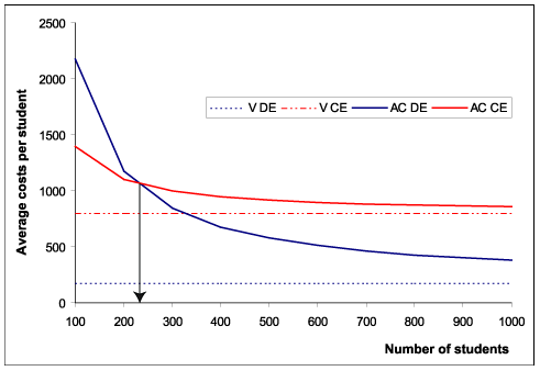
| In the above
example the red lines refer to
conventional education (CE) and the blue
lines to distance education (DE). AC DE stands for the Average Costs per Student in Distance Education and V DE for the Variable Costs per Student in Distance Education. Similarly AC CE stands for the Average Costs per Student in Conventional Education and V CE for the Variable Costs per Student in Conventional Education. The interpretation of the figure is the following: Since V DE is smaller than V CE and AC CE cannot fall below V CE, the graph of AC DE will, if student numbers are large enough, fall below the graph of AC CE (towards V DE). At the intersection point you find a downward pointing arrow which marks the break-even point. The break even point marks the number of students, beyond which (in this case) AC DE undercuts AC CE. |
It is important to note that AC cannot fall below V, however large the number of students becomes. The variable costs per student therefore represent a bottom line, below which the average costs per student cannot fall. This implies an important strategic guideline:
To lower average costs per student keep variable cost per student low.
The other strategic guideline has already been mentioned:
To bring the average cost per student down, increase the number of students.
This guideline needs some additional comment. The cube in Figure 2 shows that economies of scale vary according to the number of students already enrolled. The higher the number of students, the lower the average costs reduction effect of including another student. Hence you have to judge whether it makes sense to increase student numbers when economies of scale are already largely exhausted.
Of course, the number of students cannot be increased at will. You need to attract students and marketing efforts themselves are a cost factor and may not succeed in increasing numbers at an economic cost. Students may prefer multi-media courses with high level of learner support. If you want to offer this in order to attract further students you will need to increase V or F or both. Hence, it is important to keep in mind that N, F, V are not independent. The behavior of N is influenced by V and F. If you lower one of these parameters, students may walk away from your course and the plan to lower average costs may backfire, because the lower number of students means that fixed costs can be spread only over fewer numbers such that average cost per student will rise, possibly initiating a vicious circle.
Perraton's
Costing Cube
Perraton
(2000, p.137) has portrayed the relation between volume, media
sophistication and the interactivity. His cube (Figure 2) has
three dimensions and the arrows show the direction of reducing cost per
student.
Figure
2: Perraton's Costing Cube
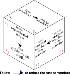
In fact, Perraton's
visualization is very close to the average cost formula. The fixed costs
in distance education are generally related to media sophistication, the
variable cost per student is strongly influenced by the level of interactivity.
(The cube is slightly modified. The original cube speaks only about face-to-face
tuition. However, meanwhile we can sustain teacher student interaction
at a distance (e.g. videoconferencing, online conferencing). But all these
forms of interactivity between students and teacher, irrespective of the
technology used, claim the teacher's time and increase variable costs.
) The Internet and videoconferencing influence the cost per student as
much as face-to-face tuition does. The number of students, varying from
few to many, is explicitly referred to in both models.
Marginal costs
We need to include a definition of marginal costs since the term is part
of the language of ODL.
Strictly speaking marginal cost means the cost of including one more student in your system.
We can express this
like this in mathematical language:
MC = TC (N + 1 )- TC (N) = [FC + V x (N + 1)] - [FC + V x N] = FC
- FC + V x (N + 1) - V x N = V
Where MC: Marginal Costs
The equation shows that the cost of including one more student in your
system is equal to the variable cost per student. The interesting point
here is that fixed costs do not impact on marginal costs. Offering something
at marginal costs therefore strictly speaking means to offer it at a price
that makes no contribution to fixed costs.
Fixed costs in ODL
are mainly related to development costs. Saying you offer something at
marginal costs often implies that you are willing to write-off the development
costs.
Semivariable costs
We have treated fixed costs and variable costs so far as a binary distinction.
This means any cost driver can either be treated as fixed cost or as variable
cost per student, as F or as V. This is a little unrealistic. In practice,
many costs are semivariable Such costs are fixed up to a certain
threshold volume.
For example, you can increase the number of students in an online seminar without adding another class as long as the number of students is below the maximum class size. Beyond this size you need to start a new class and employ an additional tutor.
The graph of a semi-variable cost takes the form of a step function: within limits you may increase volume of activity (i.e. number of students) without raising costs. At a certain point costs will jump.
Formally, we define
semivariable cost function as follows:
SV = [N/G] x SN
| Where: | |
|
SV
=
|
Semivariable
Cost
|
|
G
=
|
Group
size
|
|
V
=
|
Variable
costs per student
|
|
N
=
|
number
of students
|
|
[N/G]
=
|
Number
of groups (the square brackets signify the process of rounding )
|
|
SN
=
|
Semivariable
Cost per Group
|
Note that the number of groups (or classes) needed is defined by the number of students in the system and the maximum group size.
Theoretically, it
can be argued that all costs are semi-variable Most cost drivers are to
some extent affected by an increase in the volume of activity if only
the increase is big enough. It may be that the concept of sem-ivariable
costs has been ignored in ODL for so long because ODL was largely seen
as 'individual studies'. Nowadays it is increasingly possible to teach
classes at a distance. In this case the notion of semi-variable cost as
distinct from fixed and variable costs per student becomes more and more
important.
Total Costs = Fixed costs + Semivariable costs + Variable costs
TC = F + [N/G] x SN + V x N
|
Where:
|
|
|
TC
=
|
Total
Costs
|
|
F
=
|
Fixed
Costs
|
|
SN
=
|
Semivariable
Cost per Group
|
|
N
=
|
number
of students
|
|
SN
x [N/G] =
|
Semivariable
costs (i.e. Semivariable cost per group x number of groups)
|
|
V
x N =
|
Variable
costs (i.e. Variable cost per student x number of students)
|
|
|
Activity
A11:
Exploring the effects of group size (TC) |
||||||||||||||
|
|||||||||||||||
This leads to a modification of average costs also:
AC = TC/N
AC = F/N + ([N/G] x SN) / N + (VxN)/N
AC = F/N + SN/G + V
|
|
Activity
A12:
Exploring the effects of group size (AC) |
| This
activity looks at the effect of group size on the average cost equation.
1. Use the spreadsheet Activity 12 for this. 2. Try different group sizes to see their effect on average cost. The effects of group size on the graph are generally less visible. Click here |
|
Unit costs
Another useful concept is unit costs. You have seen that various cost drivers can be seen as variable cost per student, e.g.:
![]() print costs per student
print costs per student
![]() postage costs per student.
postage costs per student.
In order to keep unit costs low you need to control all the items that contribute to unit cost per student.
The main lessonthat
we can draw from our study of semi-variable costs is that larger group
sizes lead to greater cost efficiency. The drawback is that this reduces
the level of interactivity, a feature, which many see as an important
indicator of quality.
The generic costing template and the fixed costs/variable
costs distinction
How does the generic
costing template relate to the distinction between fixed and variable
costs? Table 8 below classifies some cost drivers.
|
DIRECT
COSTS
|
INDIRECT
COSTS
|
||
|
of
development
|
of
presentation
|
overheads
|
|
| Fixed costs | Authoring a text | Director's salary | |
| Variable costs per student | Marking of TMAs | Help desk | |
Summary and caveat:
| 1. | ODL has a different cost-structure than conventional education. |
| 2. | Cost-structure in this context refers to the composition of fixed and variable costs in the total or average cost formula. |
| 3. | ODL has a generally lower variable cost per student. This is its strategic advantage. Even though often ODL may require a higher up-front investment, these higher costs can be spread across many learners. |
| 4. | The high level of fixed costs is often seen as a guarantee for quality. The rationale for expecting ODL to be more cost-effective than conventional teaching is the combination of comparatively low variable costs per student and high fixed costs safeguarding quality (effectiveness). High quality and low costs, according to this line of thinking, can only be achieved in large systems which have a further positive and intended effect: increasing access. |
| 5. | One further comment: The efficiency path would lead to lower average cost per students. Given the enormous demand for education (and the 'perverse way' of rising unit costs), the capacity of distance education to bring down average costs per student is closely related to its remit to broaden access to education. Especially, in developing countries coping with large numbers is one of the main reasons to turn to distance education (Perraton, 2000). However, planners should be aware that lowering average costs per student in this model is achieved by expanding the system, which, in turn, raises total costs. (This caveat to any cost-analysis, exclusively singing the praises of distance education for lowering unit costs, is forcefully developed in Butcher & Roberts (2004).): |
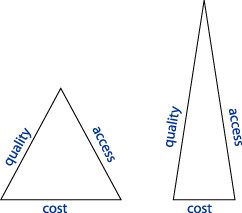
John Daniel portrays
these expectations by his eternal triangles as in Figure 3. According
to Daniel
(2001) the cost structure of ODL allows costs to be reduced while
at the same time increasing access and quality. This reflects our theoretical
expectations, but it makes assumptions that may not apply in every context.
Figure
3: The cost-quality-access triangle
![]()